


Mataupu
If you need to visually present information, then it is very convenient to do this using conditional formatting. The user who uses this service saves a huge amount of energy and time. To get the necessary information, a quick view of the file is enough.
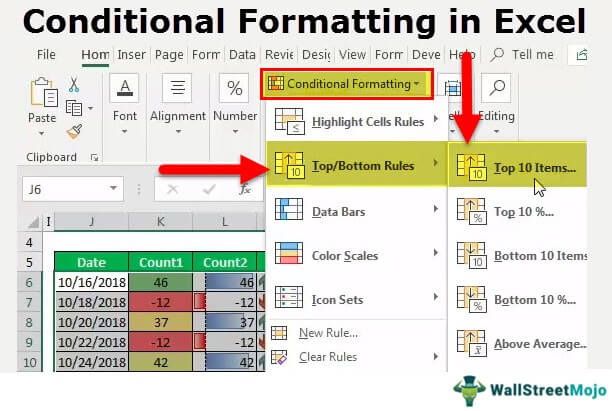
How to do conditional formatting in Excel
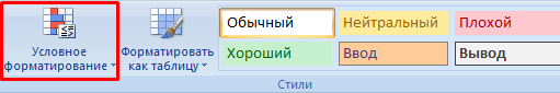
You can find “Conditional Formatting” on the very first tab of the ribbon by going to the “Styles” section.
Next, you need to find the arrow icon a little to the right with your eye, move the cursor to it. Then the settings will open, where you can flexibly configure all the necessary parameters.
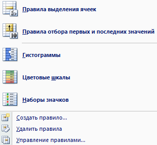
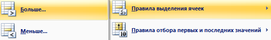
Next, you need to select the appropriate operator to compare the desired variable with a number. There are four comparison operators – greater than, less than, equal to, and between. They are listed in the rules menu.
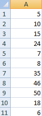
Next, we specified a series of numbers in the range A1:A11.
Let’s format a suitable data set. Then we open the “Conditional Formatting” settings menu and set the required data selection criteria. In the case of us, for example, we will select the criterion “More”.
A window with a set of options will open. In the left part of the window there is a field in which you need to specify the number 15. In the right part, the method for highlighting information is indicated, provided that it meets the previously specified criterion. The result will be displayed immediately.
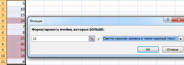
Next, complete the configuration with the OK button.
What is conditional formatting for?
To a certain extent, we can say that it is a tool, after learning which working with Excel will never be the same. This is because it makes life much easier. Instead of manually setting the formatting of a cell that matches a certain condition each time, and also trying to check it yourself for compliance with this criterion, you just need to set the settings once, and then Excel will do everything itself.
For example, you can make all cells that contain a number greater than 100 turn red. Or, determine how many days are left until the next payment, and then color in green those cells in which the deadline is still not far enough away.
Seʻi tatou faia se faʻataʻitaʻiga.
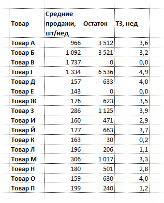
This table shows the inventory that is in stock. It has columns. as a product, average sales (measured in units per week), stock and how many weeks of this product left.
Further, the task of the purchasing manager is to determine those positions, the replenishment of which is necessary. To do this, you need to look at the fourth column from the left, which records the stock of goods by week.
Suppose the criterion for determining a cause for panic is less than 3 weeks of inventory. This indicates that we need to prepare an order. If the stock of goods is less than two weeks, then this indicates the need to urgently place an order. If the table contains a huge number of positions, then manually checking how many weeks are left is quite problematic. Even if you use the search. And now let’s see what the table looks like, which highlights scarce goods in red.
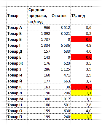
And indeed, it is much easier to navigate.
True, this example is educational, which is somewhat simplified compared to the real picture. And the saved seconds and minutes with the regular use of such tables turn into hours. Now it’s just enough to look at the table to understand which goods are in short supply, and not spend hours analyzing each cell (if there are thousands of such commodity items).
If there are “yellow” goods, then you need to start buying them. If the corresponding position is red, then you need to do it immediately.
By value of another cell
Now let’s take a look at the following practical example.
Suppose we have such a table, and we are faced with the task of highlighting rows containing certain values.
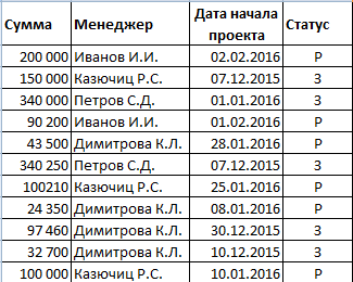
So, if the project is still being executed (that is, it has not yet been completed, therefore it is marked with the letter “P”), then we need to make its background red. Completed projects are marked in green.
Our sequence of actions in this situation will be as follows:
- Select a range of values.
- Click on the “Conditional Formatting” – “Create Rule” button.
- Please note that in our case, you need to apply the formula in the form of a rule. Next, we use the function IFto highlight matching lines.
Next, fill in the lines as shown in this picture.
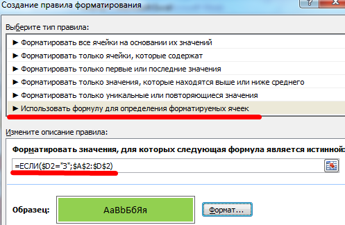
Taua! Strings must be referenced absolutely. If we refer to a cell, then in this case it is mixed (with column fixation).
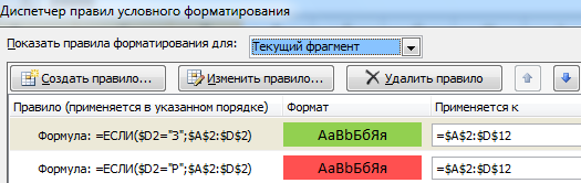
Similarly, a rule is created for those work projects that have not been completed to date.
This is what our criteria look like.
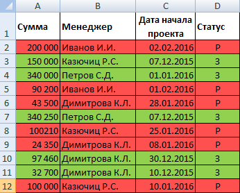
And finally, we have such a database as a result.
Multiple Conditions
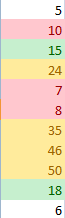
For clarity, let’s take the range A1:A11 from the table to demonstrate how, in a real practical example, you can use several conditions to determine the cell formatting.
The conditions themselves are as follows: if the number in the cell exceeds the value 6, then it is highlighted in red. If it is green, then the color is green. And finally, the largest numbers, more than 20, will be highlighted in yellow.
There are several ways how conditional formatting is carried out according to several rules.
- Method 1. We select our range, after which, in the conditional formatting settings menu, select such a cell selection rule as “More”. The number 6 is written on the left, and formatting is set on the right. In our case, the fill should be red. After that, the cycle is repeated twice, but other parameters are already set – more than 10 and green color and more than 20 and yellow color, respectively. You will get such a result.

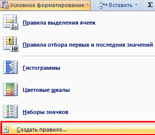
12 - Method 2. Go to the main settings menu of the Excel “Conditional Formatting” tool. There we find the “Create Rule” menu and left-click on this item.
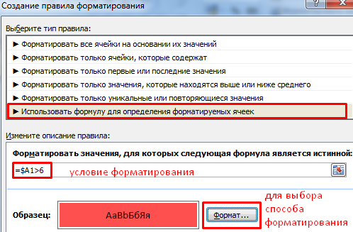
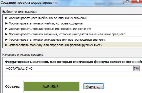
13 After that, Next, select the item “Use formula …” (highlighted in the figure with a red frame) and set the first condition. After that, click on OK. And then the cycle is repeated for subsequent conditions in the same way as described above, but the formula is used.
14
It is important to take this into account. In our example, some cells match several criteria at once. Excel resolves this conflict as follows: the rule that is above is applied first.
And here is a screenshot for better understanding.
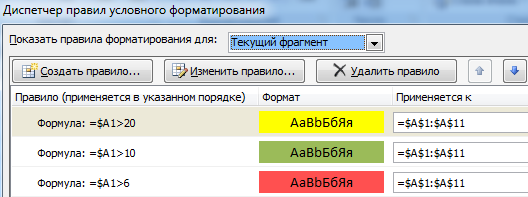
For example, we have the number 24. It meets all three conditions at the same time. In this case, there will be a fill that meets the first condition, despite the fact that it falls more under the third. Therefore, if it is important that numbers above 20 be filled with yellow, the third condition must be put in first place.
Conditional Date Formatting
Now let’s see how conditional formatting works with dates. We have such a cool range.
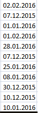
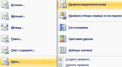
In this case, you need to set a conditional formatting rule such as “Date”.
After that, a dialog box opens with a whole set of conditions. You can get acquainted with them in detail in this screenshot (they are listed on the left side of the screen in the form of a list).
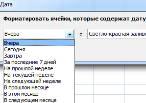
We just have to choose the appropriate one and click on the “OK” button.
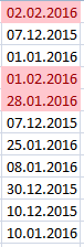
We see that those dates that refer to the last week at the time this range was drawn were highlighted in red.
Fa'aaogā fua fa'atatau
The set of standard conditional formatting rules is quite large. But situations are different, and the standard list may not be enough. In this case, you can create your own formatting rule using a formula.
To do this, click the “Create Rule” button in the conditional formatting menu, and then select the item displayed in the screenshot.
Rows (by cell value)
Suppose we need to highlight the row that contains a cell with a certain value. In this case, we need to perform the same sequence of actions as above, but for strings. That is, you can choose which range the conditional formatting should apply to.
How to create a rule
To create a rule, you must use the appropriate option in the “Conditional Formatting” section. Let’s look at a specific sequence of actions.
First you need to find the “Conditional Formatting” item on the ribbon on the “Home” tab. It can be recognized by the characteristic multi-colored cells of different sizes with a picture next to it with a crossed out equal sign.

There is a “Create Rule” button. You can also click the “Manage rules” button, after which a dialog box will open, through which you can also create a rule by clicking the corresponding button in the upper left corner.
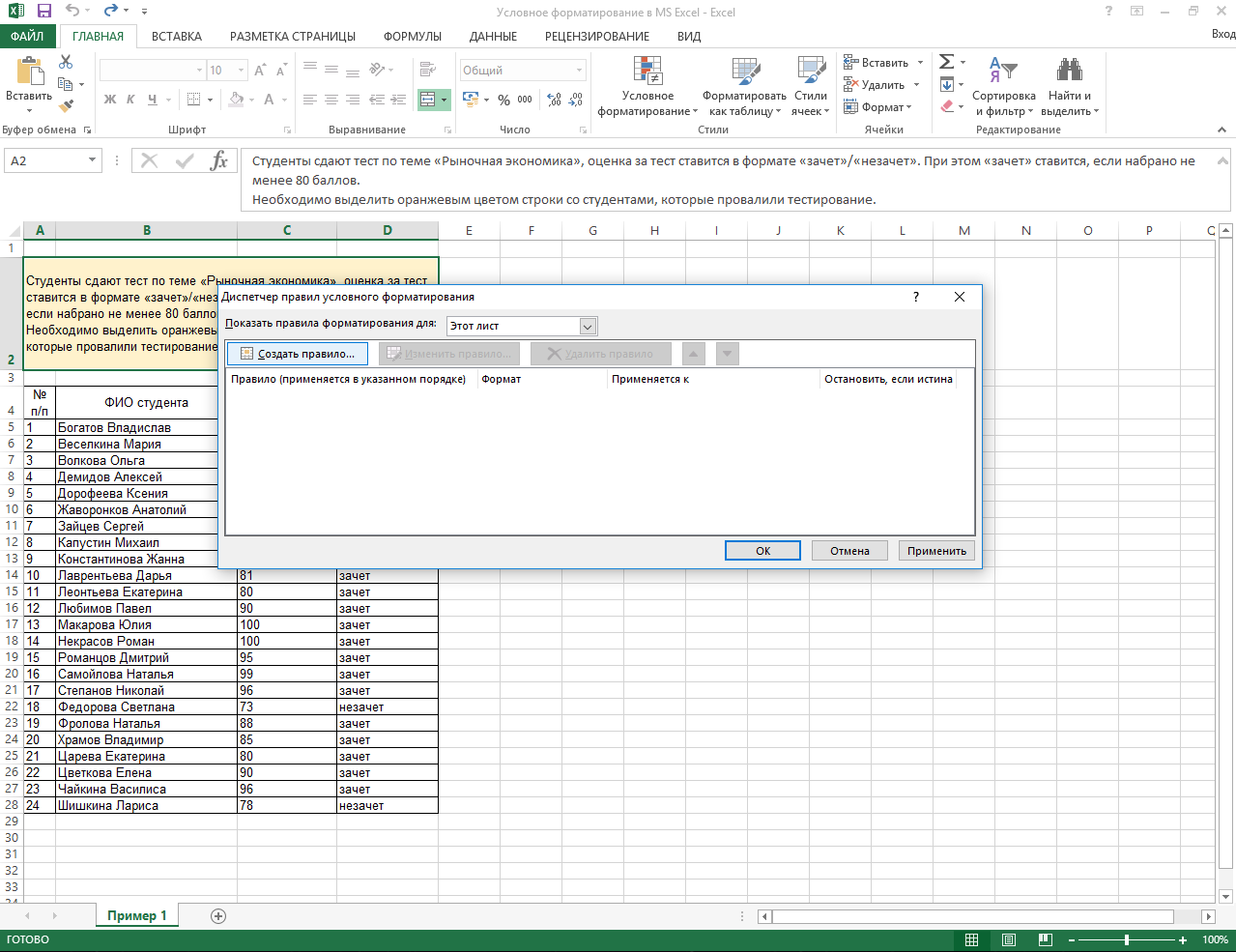
You can also see in this window those rules that have already been applied.
Tulafono filifili sela
Okay, we talk so much about how to create rules, but what is it? The cell selection rule refers to the features that are taken into account by the program to decide how to format the cells that fit them. For example, conditions can be greater than a certain number, less than a certain number, a formula, and so on. There is a whole set of them. You can familiarize yourself with them and practice their use “in the sandbox”.
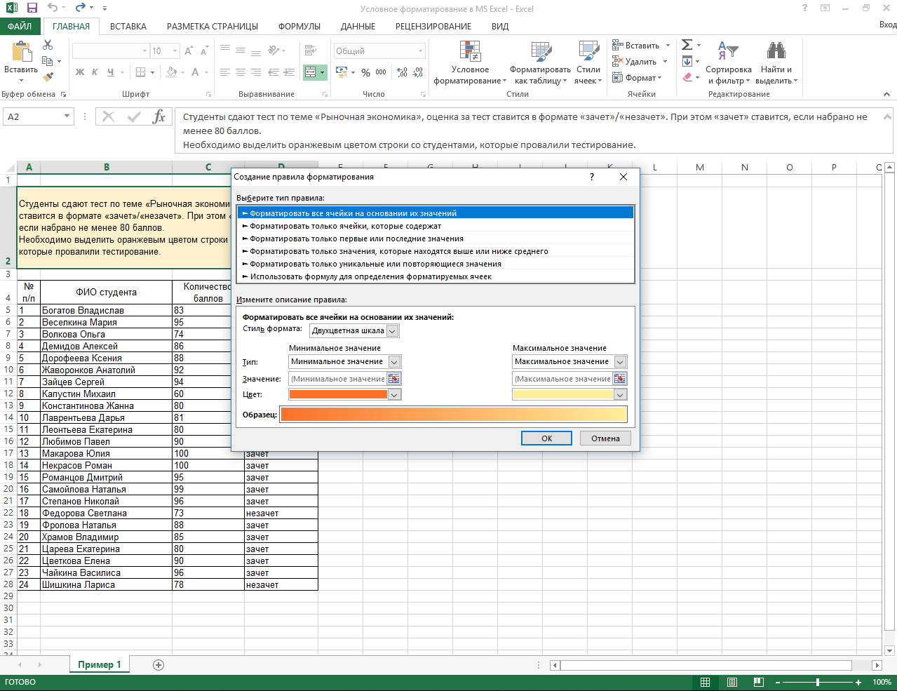
Formatting all cells based on their values
A person can independently set the range: a whole line, the entire document, or a single cell. The program can only focus on the value of one cell. This adds flexibility to the process.
Format only unique or duplicate cells
There are a large number of rules directly wired into the program. You can get acquainted with them in the “Conditional Formatting” menu. In particular, in order for formatting to apply exclusively to duplicate values or only to unique ones, there is a special option – “Duplicate values”.
If you select this item, a window with settings opens, where you can also choose the opposite option – select only unique values.
Format values in the range below and above average
To format values below or above average, there is also a special option in the same menu. But you need to select another submenu – “Rules for selecting the first and last values”.
Formatting only the first and last values
In the same submenu, it is possible to highlight only the first and last values with a special color, font and other formatting methods. According to the standard, there is an option to select the first and last ten elements, as well as 10% of the total number of cells included in this range. But the user can independently determine how many cells he needs to select.
Formatting only cells with specific content
To format only cells with specific content, you must select the Equal To or Text Contains formatting rule. The difference between them is that in the first case, the string must match the criterion completely, and in the second, only partially.
As you can see, conditional formatting is a multifunctional feature of the Excel program that gives a huge number of advantages to the person who has mastered it. We know that at first glance, all this may seem complicated. But in fact, hands are drawn to it as soon as it appears to highlight a certain piece of text in red (or format it in any other way), based on its content or in accordance with another criterion. This function is included in the basic set of Excel knowledge, without it even amateur work with spreadsheets and databases is impossible.