


Mataupu
Chart Wizard was removed from Excel 2007 and never returned in later versions. In fact, the whole system of working with diagrams was changed, and the developers did not consider it necessary to modernize the diagram wizard and related tools.
I must say that the new system for working with charts is deeply integrated into the new interface of the Menu Ribbon and is much easier to work with than the wizard that preceded it. The setup is intuitive and at every step you can see a preview of your diagram before making any changes.
Comparison of “Chart Wizard” and modern tools
For those who are used to the chart wizard, we want to say that when working with the Ribbon, all the same tools are available, usually in no more than a couple of mouse clicks.
In older versions of Excel, after clicking on the menu faaofi (Faaofiofi) > Ata (Chart) wizard showed four dialog boxes in sequence:
- Ituaiga siata. Before you select data for a chart, you need to select its type.
- Chart data source. Select the cells that contain the data to plot the chart and specify the rows or columns that should be shown as data series on the chart.
- Chart options. Customize formatting and other chart options such as data labels and axes.
- aoga ata. Select either an existing sheet or create a new sheet to host the chart you are creating.
If you need to make some changes to an already created diagram (how could it be without it ?!), then you can again use the diagram wizard or, in some cases, the context menu or menu faavaa (Format). Starting with Excel 2007, the process of creating charts has been simplified so much that the Chart Wizard is no longer needed.
- Fa'ailoga fa'amaumauga. Due to the fact that at the very beginning it is determined what data will be used to build the graph, it is possible to preview the diagram in the process of creating it.
- Select a chart type. I luga o le Advanced tab faaofi (Insert) select the chart type. A list of subtypes will open. By hovering the mouse over each of them, you can preview how the graph will look based on the selected data. Click on the selected subtype and Excel will create a chart on the worksheet.
- Customize the design and layout. Click on the created chart – in this case (depending on the version of Excel) two or three additional tabs will appear on the Ribbon. Tabs Fausia (Design), faavaa (Format) and in some versions sāuniga (Layout) allow you to apply various styles created by professionals to the created diagram, simply by clicking on the corresponding icon on the Ribbon.
- Customize di elementsagrams. To access the parameters of a chart element (for example, axis parameters), just right-click on the element and select the desired command from the context menu.
Example: Creating a histogram
We create a table on the sheet with data, for example, on sales in various cities:
In Excel 1997-2003
Kiliki i le lisi faaofi (Faaofiofi) > Ata (Chart). In the wizard window that appears, do the following:
- Ituaiga siata (Chart Type). Click siata pa (Column) and select the first of the proposed subtypes.
- Source yesdata charts (Chart Source Data). Enter the following:
- mamao (Data range): enter B4: C9 (highlighted in pale blue in the figure);
- Rows in (Series): select koluma (columns);
- I luga o le Advanced tab Lisi (Series) in the field X axis signatures (Category labels) specify a range A4:A9.
- Filifiliga Siata (Chart Options). Add a heading “Sales by Metropolitan Area» and the legend.
- Chart placement (Chart Location). Check option Place chart on sheet > iai (As object in) and select Pepa 1 (Sheet1).
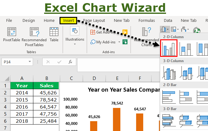
In Excel 2007-2013
- Select a range of cells with the mouse B4: C9 (highlighted in light blue in the figure).
- I luga o le Advanced tab faaofi (Faaofi) kiliki Fa'aofi le histogram (Insert Column Chart).
- filifili Histogram ma fa'avasegaga (2-D Clustered Column).
- In the tab group that appears on the ribbon Galue ma siata (Chart Tools) open tab Fausia (Design) ma lolomi Filifili faamatalaga (Select Data). In the dialog box that appears:
- I le Fa'ailoga tu'usa'o (vaega) (Horizontal (category) labels) click liuga (Edit) on A4:A9ona fetaomi lea OK;
- liuga laina1 (Series1): in the field igoa laina (Series name) select cell B3;
- liuga laina2 (Series2): in the field igoa laina (Series name) select cell C3.
- In the created chart, depending on the version of Excel, either double-click on the chart title, or open the tab Galue ma siata (Chart Tools) > sāuniga (Layout) and enter “Sales by Metropolitan Area".
O le a le mea e fai?
Take some time to explore the available chart options. See what tools are on the group tabs Galue ma siata (ChartTools). Most of them are self-explanatory or will show a preview before a selection is made.
After all, is there a better way to learn than practice?