E faʻafefea ona fatuina se siata Gantt i Excel?

If you are asked to name the three most important components of Microsoft Excel, which ones would you name? Most likely, sheets on which data is entered, formulas that are used to perform calculations, and charts with which data of a different nature can be represented graphically.

I am sure that every Excel user knows what a chart is and how to create it. However, there is a type of chart that is shrouded in obscurity for many – Siata siata. This quick guide will explain the main features of a Gantt chart, tell you how to make a simple Gantt chart in Excel, tell you where to download advanced Gantt chart templates, and how to use the Project Management online service to create Gantt charts.

• O le a le Gantt Chart?
• E faʻafefea ona fatuina se siata Gantt i Excel?
• Gantt siata mamanu

O le a le Gantt Chart?

Siata siata named after Henry Gantt, an American engineer and management consultant who came up with the diagram in 1910. The Gantt chart in Excel represents projects or tasks as a cascade of horizontal bar charts. The Gantt chart shows the broken down structure of the project (start and finish dates, various relationships between tasks within the project) and thus helps to control the execution of tasks in time and according to the intended benchmarks.

How to Create a Gantt Chart in Excel 2010, 2007 and 2013

Unfortunately, Microsoft Excel does not offer a built-in Gantt chart template. However, you can quickly create one yourself using the bar chart functionality and a little bit of formatting.

Follow these steps carefully and it will take no more than 3 minutes to create a simple Gantt chart. In our examples, we are creating a Gantt chart in Excel 2010, but the same can be done in Excel 2007 and 2013.

Step 1. Create a project table

First of all, we will enter the project data into an Excel sheet. Write each task on a separate line and build a project breakdown plan by specifying amata aso (Start date), faauuga (end date) and umi (Duration), that is, the number of days it takes to complete the task.

Fautuaga: Only the columns are needed to create a Gantt chart Aso amata и umi. However, if you also create a column End date, then you can calculate the duration of the task using a simple formula, as seen in the figure below:

Step 2. Build a regular Excel bar chart based on the “Start date” column database

Start building a Gantt chart in Excel by creating a simple fa'aputu siata pa:

• Fa'ailoga se vaega Amata Aso along with the column heading, in our example it is B1: B11:. It is necessary to select only cells with data, and not the entire column of the sheet.
• I luga o le Advanced tab faaofi (Insert) under Charts, click Fa'aofi le siata pa (Bar).
• In the menu that opens, in the group Puleaina (2-D Bar) click Pule Faaputu (Pa Fa'aputu).

As a result, the following chart should appear on the sheet:

Manatua: Some of the other instructions for creating Gantt charts suggest that you first create an empty bar chart and then fill it with data, as we will do in the next step. But I think that the method shown is better because Microsoft Excel will automatically add one row of data and this way we will save some time.

Step 3: Add Duration Data to the Chart

Next, we need to add one more data series to our future Gantt chart.

1. Right-click anywhere in the diagram and in the context menu click Filifili faamatalaga (Select Data).A dialog box will open Filifilia o se punavai o faamatalaga (Select Data Source). As you can see in the figure below, the column data amata Aso already added to the field O mea taua (laina) (Legend Entries (Series). Now you need to add column data here umi.
2. Kiliki le faʻamau faʻaopoopo (Add) to select additional data (Duration) to display on the Gantt chart.
3. I le faamalama matala Suiga laina (Edit series) do this:
   • I le igoa laina (Series name) enter “Duration” or any other name you wish. Or you can place the cursor in this field and then click on the title of the corresponding column in the table – the title that is clicked on will be added as the series name for the Gantt chart.
   • Click the range selection icon next to the field O tulaga faatauaina (Tulaga taua).
4. Fa'amalama talanoaga Suiga laina (Edit series) will decrease. Highlight data in a column umiby clicking on the first cell (in our case it is D2) and dragging down to the last data cell (D11). Make sure you don’t accidentally select a heading or some empty cell.
5. Press the range selection icon again. Dialog window Suiga laina (Edit series) will be expanded again and the fields will appear igoa laina (Igoa o le faasologa) ma O tulaga faatauaina (Series values). Click OK.
6. We’ll go back to the window again Filifilia o se punavai o faamatalaga (Select Data Source). Now in the field O mea taua (laina) (Legend Entries (Series) we see a series amata Aso and a number umi. Naʻo le kiliki OK, and the data will be added to the chart.

The diagram should look something like this:

Step 4: Add Task Descriptions to the Gantt Chart

Now you need to show a list of tasks on the left side of the diagram instead of numbers.

1. Right-click anywhere in the plotting area (the area with blue and orange stripes) and in the menu that appears, click Filifili faamatalaga (Select Data) to reappear the dialog box Filifilia o se punavai o faamatalaga (Filifili Fa'amatalaga Punaoa).
2. In the left area of ​​the dialog box, select amata Aso Ma kiliki le liuga (Edit) in the right area of ​​the window titled Fa'ailoga tu'usa'o (vaega) (Horizontal (Category) Axis Labels).
3. A small dialog box will open Axis labels (Axis labels). Now you need to select tasks in the same way as in the previous step we selected data on the duration of tasks (Durations column) – click the range selection icon, then click on the first task in the table and drag the selection with the mouse down to the last task. Remember that the column heading should not be highlighted. Once you’ve done that, click the range selection icon again to bring up the dialog box.
4. Oomi faʻalua OKto close all dialog boxes.
5. Delete the chart legend – right-click on it and in the context menu click aveese (Tape).

At this point, the Gantt chart should have task descriptions on the left side and look something like this:

Step 5: Converting a Bar Chart to a Gantt Chart

At this stage, our chart is still a stacked bar chart. To make it look like a Gantt chart, you need to format it correctly. Our task is to remove the blue lines so that only the orange parts of the graphs, which represent the tasks of the project, remain visible. Technically, we won’t remove the blue lines, we’ll just make them transparent and therefore invisible.

1. Click on any blue line on the Gantt chart, and all of them will be selected. Right-click on the selection and in the context menu click Fa'asologa o fa'amaumauga (Fa'asologa o Fa'amaumauga).
2. In the dialog box that appears, do the following:
   • I le vaega faʻatumu (Faatumu) filifili Leai se faʻatumuina (Leai Faatumu).
   • I le vaega tuāʻoi (Border Color) select leai ni laina (No Line).

Manatua: Do not close this dialog box, you will need it again in the next step.

3. The tasks on the Gantt chart that we built in Excel are in reverse order. We’ll fix that in a moment. Click on the list of tasks on the left side of the Gantt chart to highlight the category axis. A dialog box will open Fuafuaga Axis (Format Axis). In chapter Fa'amaufa'ailoga axis (Axis Options) siaki le pusa Toe fesuia'i le faasologa o vaega (Categories in reverse order), then close the window to save your changes.As a result of the changes we just made:
   • The tasks on the Gantt chart are in the correct order.
   • The dates on the horizontal axis have moved from the bottom to the top of the chart.

The chart becomes similar to a regular Gantt chart, right? For example, my Gantt chart now looks like this:

Step 6. Customizing the Gantt Chart Design in Excel

The Gantt chart is already taking shape, but you can add a few more finishing touches to make it really stylish.

1. Remove the empty space on the left side of the Gantt chart

When building a Gantt chart, we inserted blue bars at the beginning of the chart to show the start date. Now the void that remains in their place can be removed and the task strips can be moved to the left, closer to the vertical axis.

• Right click on the first column value amata Aso in the table with source data, in the context menu select Fa'asologa o sela > nūmera > Aoao (Format Cells > Number > General). Memorize the number you see in the field faʻatusa (Sample) is the numeric representation of the date. In my case this number 41730. As you know, Excel stores dates as numbers equal to the number of days dated January 1, 1900 before this date (where January 1, 1900 = 1). You don’t need to make any changes here, just click faalēaogāina (Faaleaogaina).
• On the Gantt chart, click on any date above the chart. One click will select all the dates, after that right-click on them and in the context menu click Fuafuaga Axis (Format Axis).
• I luga o le lisi le faataamilosaga tua (Axis Options) change the option aupito itiiti (Minimum) on nūmera (Fixed) and enter the number you remembered in the previous step.

2. Adjust the number of dates on the axis of the Gantt chart

Here, in the dialog box Fuafuaga Axis (Format Axis) that was opened in the previous step, change the parameters Vaega tetele (Major united) и Vaevaega vaeluagalemu (Minor unit) of nūmera (Fixed) and enter the desired values ​​for the intervals on the axis. Usually, the shorter the time frames of the tasks in the project, the smaller the division step is needed on the time axis. For example, if you want to show every second date, then enter 2 mo parameter Vaega tetele (Major unit). What settings I made – you can see in the picture below:

Fautuaga: Play around with the settings until you get the desired result. Don’t be afraid to do something wrong, you can always revert to the default settings by setting the options to Faʻamataʻu (Auto) in Excel 2010 and 2007 or by clicking toe setiina (Reset) in Excel 2013.

3. Remove the extra empty space between the stripes

Arrange the task bars on the chart more compactly, and the Gantt chart will look even better.

• Select the orange bars of the graphs by clicking on one of them with the left mouse button, then right-click on it and in the menu that appears, click Fa'asologa o fa'amaumauga (Fa'asologa o Fa'amaumauga).
• I le pusa talanoa Fa'asologa o fa'amaumauga (Format Data Series) set the parameter to laina fa'atasi (Series Overlap) value 100% (slider moved all the way to the right), and for the parameter Fa'amama le itu (Gap Width) value 0% or almost 0% (slider all the way or almost all the way to the left).

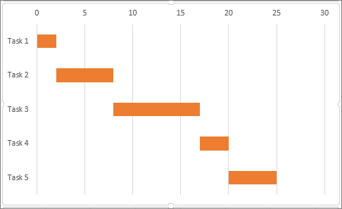
And here is the result of our efforts – a simple but quite accurate Gantt chart in Excel:

Remember that an Excel chart created in this way is very close to a real Gantt chart, while retaining all the convenience of Excel charts:

• The Gantt chart in Excel will resize when tasks are added or removed.
• Change the start date of the task (Start date) or its duration (Duration), and the schedule will immediately automatically reflect the changes made.
• The Gantt chart created in Excel can be saved as an image or converted to HTML format and published on the Internet.

FAUTUAGA:

• Customize the appearance of your Gantt chart by changing fill options, borders, shadows, and even using 3D effects. All of these options are available in the dialog box. Fa'asologa o fa'amaumauga (Format Data Series). To call this window, right-click on the chart bar in the chart plotting area and in the context menu click Fa'asologa o fa'amaumauga (Fa'asologa o Fa'amaumauga).
• If the design style created is pleasing to the eye, then such a Gantt chart can be saved in Excel as a template and used in the future. To do this, click on the diagram, open the tab Fausia (Design) ma lolomi Fa'asaoina e fai ma fa'ata'ita'iga (Save as Template).

Download sample Gantt chart

Gantt chart template in Excel

As you can see, building a simple Gantt chart in Excel is not difficult at all. But what if a more complex Gantt chart is required, in which task shading depends on the percentage of its completion, and project milestones are indicated by vertical lines? Of course, if you are one of those rare and mysterious creatures that we respectfully call the Excel Guru, then you can try to make such a diagram yourself.

However, it will be faster and easier to use pre-made Gantt chart templates in Excel. Below is a brief overview of several project management Gantt chart templates for various versions of Microsoft Excel.

Microsoft Excel 2013 Gantt Chart Template

This Gantt chart template for Excel is called Fuafuaga o le Poloketi (Gantt Project Planner). It is designed to track project progress against various metrics such as Planned start (Plan Start) и actual start (Actual Start), Planned duration (Plan Duration) и Actual Duration (Actual Duration), as well as Maea pasene (Percent Complete).

In Excel 2013, this template is available on the tab faila (File) in the window faia (New). If there is no template in this section, you can download it from the Microsoft website. No additional knowledge is required to use this template – click on it and get started.

Online Template Chart Ganta

Smartsheet.com offers an interactive online Gantt Chart Builder. This Gantt chart template is just as simple and ready to use as the previous one. The service offers a 30-day free trial, so feel free to sign up with your Google account and start creating your first Gantt chart right away.

The process is very simple: in the table on the left, enter the details of your project, and as the table fills in, a Gantt chart is created on the right.

Gantt Chart Templates for Excel, Google Sheets and OpenOffice Calc

At vertex42.com you can find free Gantt chart templates for Excel 2003, 2007, 2010 and 2013 that will also work with OpenOffice Calc and Google Sheets. You can work with these templates just like you would with any regular Excel spreadsheet. Just enter a start date and duration for each task and enter the % complete in the column % complete. To change the date range shown in the Gantt chart area, move the slider on the scroll bar.

And finally, another Gantt chart template in Excel for your consideration.

Project Manager Gantt Chart Template

Another free Gantt chart template is offered at professionalexcel.com and is called “Project Manager Gantt Chart”. In this template, it is possible to choose a view (daily or standard weekly), depending on the duration of the tracked tasks.

I hope that at least one of the proposed Gantt chart templates will suit your needs. If not, you can find a great variety of different Gantt chart templates on the Internet.

Now that you know the main features of the Gantt chart, you can continue learning it and learn how to create your own complex Gantt charts in Excel to surprise your boss and all your colleagues 🙂