E faʻafefea ona faʻaisaina se cell i se Excel formula

Often, users are faced with the need to pin a cell in a formula. For example, it occurs in situations where you want to copy a formula, but so that the link does not move up and down the same number of cells as it was copied from its original location.

In this case, you can fix the cell reference in Excel. And this can be done in several ways at once. Let’s take a closer look at how to achieve this goal.

What is an Excel link

The sheet is made up of cells. Each of them contains specific information. Other cells can use it in calculations. But how do they understand where to get the data from? It helps them make links.

Each link designates a cell with one letter and one number. A letter represents a column and a number represents a row. 

There are three types of links: absolute, relative and mixed. The second one is set by default. An absolute reference is one that has a fixed address of both a column and a column. Accordingly, mixed is the one where either a separate column or a row is fixed.

Ole auala 1

In order to save both column and row addresses, follow these steps:

1. Click on the cell containing the formula.
2. Click on the formula bar for the cell that we need.
3. Oomi le F4.

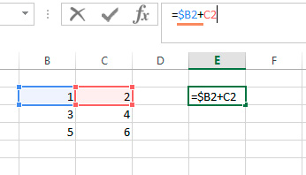
As a consequence, the cell reference will change to absolute. It can be recognized by the characteristic dollar sign. For example, if you click on cell B2 and then click on F4, the link will look like this: $B$2.

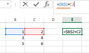
What does the dollar sign mean before the part of the address per cell?

1. If it is placed in front of a letter, it indicates that the column reference remains the same, no matter where the formula has been moved.
2. If the dollar sign is in front of the number, it indicates that the string is pinned. 

Ole auala 2

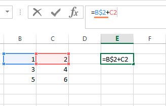
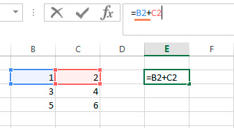
This method is almost the same as the previous one, only you need to press F4 twice. for example, if we had cell B2, then after that it will become B$2. In simple words, in this way we managed to fix the line. In this case, the letter of the column will change.

It is very convenient, for example, in tables where you need to display the contents of the second cell from the top in the bottom cell. Instead of doing such a formula many times, it is enough to fix the row and let the column change.

Ole auala 3

This is completely the same as the previous method, only you need to press the F4 key three times. Then only the reference to the column will be absolute, and the row will remain fixed.

Ole auala 4

Suppose we have an absolute reference to a cell, but here it was necessary to make it relative. To do this, press the F4 key so many times that there are no $ signs in the link. Then it will become relative, and when you move or copy the formula, both the column address and the row address will change.

Pinning cells for a large range

We see that the above methods do not present any difficulty at all to perform. But the tasks are specific. And, for example, what to do if we have several dozen formulas at once, the links in which need to be turned into absolute ones. 

Unfortunately, standard Excel methods will not achieve this goal. To do this, you need to use a special addon called VBA-Excel. It contains many additional features that allow you to perform common tasks with Excel much faster.

It includes more than a hundred user-defined functions and 25 different macros, and it is also updated regularly. It allows you to improve work with almost any aspect:

1. sela.
2. Macro
3. Functions of different types.
4. Links and arrays.

In particular, this add-in allows you to fix links in a large number of formulas at once. To do this, you must perform the following steps:

1. Filifili se vaega.
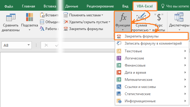
2. Open the VBA-Excel tab that will appear after installation. 
3. Open the “Functions” menu, where the “Lock formulas” option is located.
   

   

4. Next, a dialog box will appear in which you need to specify the required parameter. This addon allows you to pin a column and a column separately, together, and also remove an already existing pinning with a package. After the required parameter is selected using the corresponding radio button, you need to confirm your actions by clicking “OK”.

faataitaiga

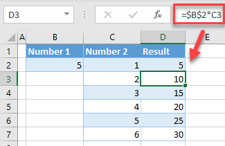
Let’s take an example to make it more clear. Let’s say we have information that describes the cost of goods, its total quantity and sales revenue. And we are faced with the task of making the table, based on the quantity and cost, automatically determine How long money we managed to earn without deducting losses.

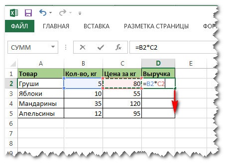
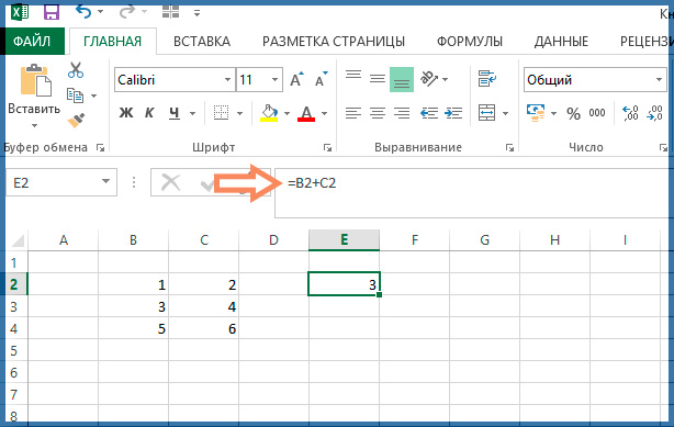
In our example, for this you need to enter the formula =B2*C2. It’s quite simple, as you can see. It is very easy to use her example to describe how you can fix the address of a cell or its individual column or row. 

Of course, in this example, you can try to drag the formula down using the autofill marker, but in this case, the cells will be automatically changed. So, in cell D3 there will be another formula, where the numbers will be replaced, respectively, by 3. Further, according to the scheme – D4 – the formula will take the form = B4 * C4, D5 – similarly, but with the number 5 and so on.

If it is necessary (in most cases it turns out), then there are no problems. But if you need to fix the formula in one cell so that it does not change when dragging, then this will be somewhat more difficult. 

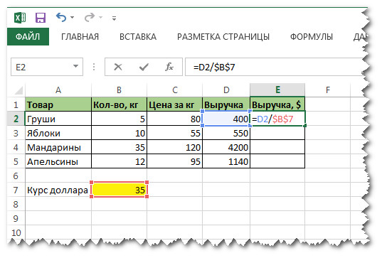
Suppose we need to determine the dollar revenue. Let’s put it in cell B7. Let’s get a little nostalgic and indicate the cost of 35 rubles per dollar. Accordingly, in order to determine the revenue in dollars, it is necessary to divide the amount in rubles by the dollar exchange rate.

Here’s what it looks like in our example.

If we, similarly to the previous version, try to prescribe a formula, then we will fail. Similarly, the formula will change to the appropriate one. In our example, it will be like this: =E3*B8. From here we can see. that the first part of the formula has turned into E3, and we set ourselves this task, but we do not need to change the second part of the formula to B8. Therefore, we need to turn the reference into an absolute one. You can do this without pressing the F4 key, just by putting a dollar sign.

After we turned the reference to the second cell into an absolute one, it became protected from changes. Now you can safely drag it using the autofill handle. All fixed data will remain the same, regardless of the position of the formula, and uncommitted data will change flexibly. In all cells, the revenue in rubles described in this line will be divided by the same dollar exchange rate.

The formula itself will look like this:

=D2/$B$7

Atu! We have indicated two dollar signs. In this way, we show the program that both the column and the row need to be fixed.

Cell references in macros

A macro is a subroutine that allows you to automate actions. Unlike the standard functionality of Excel, a macro allows you to immediately set a specific cell and perform certain actions in just a few lines of code. Useful for batch processing of information, for example, if there is no way to install add-ons (for example, a company computer is used, not a personal one).

First you need to understand that the key concept of a macro is objects that can contain other objects. The Workbooks object is responsible for the electronic book (that is, the document). It includes the Sheets object, which is a collection of all sheets of an open document. 

Accordingly, cells are a Cells object. It contains all the cells of a particular sheet.

Each object is qualified with parenthesized arguments. In the case of cells, they are referenced in this order. The row number is listed first, followed by the column number or letter (both formats are acceptable).

For example, a line of code containing a reference to cell C5 would look like this:

Workbooks(“Book2.xlsm”).Sheets(“List2”).Cells(5, 3)

Workbooks(“Book2.xlsm”).Sheets(“List2”).Cells(5, “C”)

You can also access a cell using an object Tidy. In general, it is intended to give a reference to a range (whose elements, by the way, can also be absolute or relative), but you can simply give a cell name, in the same format as in an Excel document.

In this case, the line will look like this.

Workbooks(“Book2.xlsm”).Sheets(“List2”).Range(“C5”)

It may seem that this option is more convenient, but the advantage of the first two options is that you can use variables in brackets and give a link that is no longer absolute, but something like a relative one, which will depend on the results of the calculations.

Thus, macros can be effectively used in programs. In fact, all references to cells or ranges here will be absolute, and therefore can also be fixed with them. True, it is not so convenient. The use of macros can be useful when writing complex programs with a large number of steps in the algorithm. In general, the standard way of using absolute or relative references is much more convenient. 

faaiuga

We figured out what a cell reference is, how it works, what it is for. We understood the difference between absolute and relative references and figured out what needs to be done in order to turn one type into another (in simple words, fix the address or unpin it). We figured out how you can do it immediately with a large number of values. Now you have the flexibility to use this feature in the right situations.